knitr + cactus + TwitterBootstrap + Jquery

A few notes and tips from a week of preparing some course notes.

I switched from Sweave to knitr because all the cool kids are doing it. And its better. The caching has already saved me more time than I spent switching from Sweave to knitr, which wasn't much time at all. Win

At first I was building a PDF from .Rnw sources, but then thought maybe HTML would be a better delivery platform. No need to open a PDF reader. So I figured out the .Rhtml syntax and it was done. Win.

But how to do my equations? Mathjax. Problem solved. Almost pixel-perfect equations using LaTeX syntax. Users without Javascript get the LaTeX source so its not all lost on them. Win.

Making a simple HTML file is easy enough, but I want to make a few tutorial sessions, and some other info, so I want to use a template engine. My current fave is cactus.py - you design Django templates, then write your pages to fill in sections such as 'title' or 'content' in the template, then cactus.py will build the static pages. These can then be served by a simple web server or straight from the file system. Win.

So instead of a full HTML file, I just got knitr to process a Django template chunk. However, this didn't give me the CSS for the source code syntax highlighting because there's no HEAD section in the Html. Solved by copying the knitr CSS into a file and serving it up from my template. Works fine, and serving CSS from files rather than inline in HTML is a win because now the server or client can cache it. Win.

For style and structure, I just write my templates to use styles from the Twitter Bootstrap framework. Include the CSS and JS in your template base and you have good-looking responsive pages. Sure, they look like every other Twitter Bootstrap site, but the flexibility to style them is there too. Win.

Then I figured something real cool. The R syntax highlighting wraps all functions with a span of class "functioncall". One line of jQuery can turn all those spans into hyperlinks to information from my current favourite R documentation - the R Graphical Manual. Here's some code which might get mangled by Blogger's formatting and/or my inexperience trying to stick hypertext tags into a Blogger doc:

$("span.functioncall").replaceWith(function(){return '< a href="http://rgm2.lab.nig.ac.jp/RGM2/search.php?query='+$(this).text()+'" >'+$(this).text()+'< /a >'})

Now every function links to the search for that function name. It's probably hard to link directly to the help for that function exactly, since the system would have to know what package each function was in to get to exactly the right help on the RGM, but this is a big help. Win.

So that was my weekend. Also, Chelsea FC. Win.

Reading AfriPop data

The AfriPop project aims to produce high-resolution population density estimates for Africa. This could be very useful for some of our spatial epi projects. So I thought I'd have a look.

Their methods for computing population are explained. I can't find any licensing or usage restrictions on the data, so I'll have to clear that up before doing anything serious with it. Let's download something and read it in.

The download form asks for a few details, but there's no email check (or 'I have read your terms and conditions' checkbox) so fill in as honestly as your conscience requires. You'll get a zip file to download.

When unzipped you'll have three files. For Benin these are called apben10v3 with extensions hdr, flt and prj.


The flt file is the data, the hdr is header info, and prj is projection info. Use gdalinfo to get a summary - run it on the flt file:

$ gdalinfo apben10v3.flt 

Driver: EHdr/ESRI .hdr Labelled

Files: apben10v3.flt

       apben10v3.hdr

       apben10v3.prj

[WGS84 coordinate system info here]

Origin = (0.773989957311480,12.409206711176100)

Pixel Size = (0.000833300000000,-0.000833300000000)

Corner Coordinates:

Upper Left (0.7739900,12.4092067) (0d46'26.36"E,12d24'33.14"N)

Lower Left  (0.7739900,6.2252874) (0d46'26.36"E,6d13'31.03"N)

Upper Right (3.8522002,12.4092067)(3d51' 7.92"E,12d24'33.14"N)

Lower Right (3.8522002,6.2252874) (3d51' 7.92"E,6d13'31.03"N)

Center      (2.3130951,9.3172471) (2d18'47.14"E,  9d19' 2.09"N)

Band 1 Block=3694x1 Type=Byte, ColorInterp=Undefined

  NoData Value=-9999

All pretty good. A standard ESRI file (except there's often nothing really standard about ESRI file formats). Let's read it and plot it using the raster package:

> bpop=raster("./apben10v3.flt")

> image(bpop)

Oh dear. Reading the docs about these files tells me that sometimes gdal just doesn't get it right. It said "Type=Byte", but the file is 109652696 bytes long, which is exactly 7421x3694x4 bytes. These are 4 byte values. In fact the AfriPop page says these files are "ESRI Float". Luckily there's an easy way to persuade gdal these are floats. Open up the hdr file (NOT the flt file. Don't open the flt file!) in a text editor (emacs, vi, notepad++, notepad) and add:

 pixeltype float

to the items. Then try again:

> bpop=raster("./apben10v3.flt")

> plot(bpop,asp=1)

Looks good. Note we can get away with asp=1 since we're close to the equator. Or we can give it a projection:

 projection(bpop)="+proj=tmerc"

 plot(bpop)

and that's just as good. We can also zoom in using the very nifty zoom function from the raster package:

 and inspect the data further.

Note that the raster package does a really good job of dealing with large rasters. When plotting these things it is sampling the raster file so not all of it is read into memory. I don't have a monitor capable of showing 7000x3000 pixels (yet) so raster just grabs enough to look good. But if you try and do anything with this size of raster, you will strangle your machine and it may die. Don't do this:


plot(log(bpop))

for example. Let's sample our raster down a bit for some more exploring. First I need to restart R after the last line crashed out. I'll sample down to something of the order of a few hundred pixels by a few hundred pixels by specifying the size as 500*500 - sampleRegular will work out the exact resolution, keeping the aspect ratio. It's smart like that:

> library(raster)

> bpop=raster("apben10v3.flt")

> projection(bpop)="+proj=tmerc"

> plot(bpop)

> bpop2 = sampleRegular(bpop, 500*500, asRaster=TRUE)

> bpop2

class       : RasterLayer 

dimensions  : 708, 352, 249216  (nrow, ncol, ncell)

resolution  : 0.008744915, 0.008734349  (x, y)

extent      : 0.77399, 3.8522, 6.225287, 12.40921  (xmin, xmax, ymin, ymax)

coord. ref. : +proj=tmerc +ellps=WGS84 

values      : in memory

min value   : 0 

max value   : 336.4539 

> plot(bpop2)

> plot(log(bpop2))

[Perhaps we should use 'resample' here?] Now the log plot is doable:

BUT these values are now wrong. The units of the original data are persons per grid square. Our grid squares are now bigger then the original grid squares, so more people live in them. We can correct this by scaling by the ratio of the cell sizes:

> bpop2= bpop2 * prod(res(bpop2))/prod(res(bpop))

> plot(log(bpop2))

and now we get a more correct map:

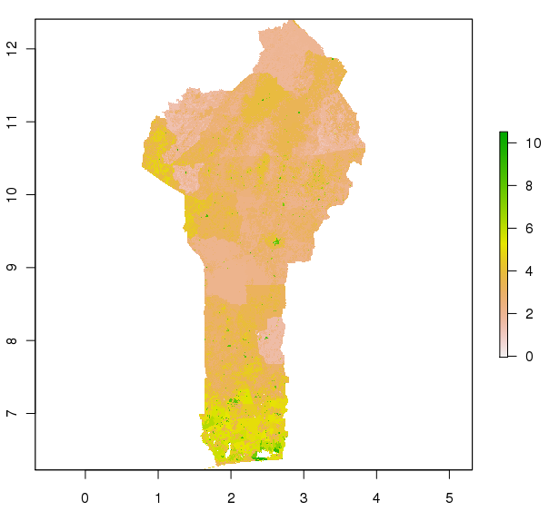
I'm not sure how 'correct' or optimal this is of downsampling population density grids is - for example the total population (sum of grid cells) will be slightly different. Perhaps it is better to rescale the sampled grid to keep the total population the same? Thoughts and musings in comments for discussion please!

optifix - optim with fixed values

So you've written your objective function, fr, and want to optimise it over the two parameters. Fire up optim and away you go:

> fr <- function(x) {   ## Rosenbrock Banana function

     x1 <- x[1]

     x2 <- x[2]

     100 * (x2 - x1 * x1)^2 + (1 - x1)^2

 }

> optim(c(-1.2,1), fr)[c("par","value")]

$par

[1] 1.000260 1.000506

$value

[1] 8.825241e-08

Great. But sometimes you only want to optimise over some of your parameters, keeping the others fixed. Let's consider optimising the banana function for x2=0.3

>  fr <- function(x) {   ## Rosenbrock Banana function

         x1 <- x[1]

         x2 <- 0.3

         100 * (x2 - x1 * x1)^2 + (1 - x1)^2

     }

> optim(-1.2, fr,method="BFGS")[c("par","value")]

$par

[1] -0.5344572

$value

[1] 2.375167

(R gripes about doing 1-d optimisation with Nelder-Mead, so I switch to BFGS)

Okay, but we had to write a new objective function with 0.3 coded into it. Now repeat for a number of values. That's a pain.

The conventional solution would be to make x2 an extra parameter of fr:

>  fr <- function(x,x2) {

         x1 <- x[1]

         100 * (x2 - x1 * x1)^2 + (1 - x1)^2

     }

and call optim with this passed in the dot-dot-dots:

> optim(-1.2,fr,method="BFGS",x2=0.3)[c("par","value")]

$par

[1] -0.5344572

$value

[1] 2.375167

Okay great. But suppose now we want to fix x1 and optimise over x2. You're going to need another objective function. Suppose your function has twelve parameters... This is becoming a pain.

You need optifix. Go back to the original 2 parameter banana function, and do:

> optifix(c(-1.2,0.3),c(FALSE,TRUE), fr,method="BFGS")

$par

[1] -0.5344572

$value

[1] 2.375167

$counts

function gradient 

      27        9 

$convergence

[1] 0

$message

NULL

$fullpars

[1] -0.5344572  0.3000000

$fixed

[1] FALSE  TRUE

Here the function call is almost the same as the 2-parameter optimisation, except with a second argument that tells which parameters to fix - and they are fixed at the values given in the first argument. The values in that argument for non-fixed parameters are starting values for the optimiser as usual.

The output is the output from the reduced optimiser. In this case it is one parameter value, but there's also a couple of other components, $fullpars and $fixed, to tell you what the overall parameter values were and which ones were fixed.

Optifix takes your objective function and your specification of what's fixed to create a wrapper round your function that only takes the variable parameters. The wrapper inserts the fixed values in the right place and calls your original function. It then calls optim with a reduced vector of starting parameters and the wrapped objective function. Hence the wrapped function is only every called with the variable parameters, and the original function is called with the variables and the fixed values.

Optifix should work on optim calls that use a supplied gradient function - it wraps that as well to produce a reduced-dimensional gradient function  for optim to work on.

Code? Oh you want the code? Okay. I've put a file in a folder on a server for you to download. Its very beta, needs testing and probably should find a package for its home. All things to do.